S2 Cheat Sheet

Sampling and Estimation

Central Limit Theorem (CLT) – For the sample mean (when it's not stated to be normally distributed and $n$ is large, $n > 1$ ), we use the CLT to assume it's normally distributed.

z = \frac{\bar{x} - \mu}{\frac{\sigma}{\sqrt{n}}}

$\bar{x}$ = sample mean
$E(\bar{x}) = \mu$ = population mean
$Var(\bar{x}) = \frac{\sigma^2}{n}$ = sample variance

Unbiased Estimator

\mu = \frac{\Sigma x}{n}

Var(x) = \frac{1}{n - 1} \left( \Sigma x^2 - \frac{(\Sigma x)^2}{n} \right) = s^2

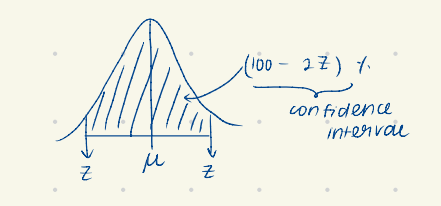
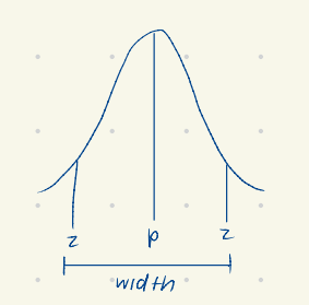
Confidence Interval

The region which has the highest probability of containing the population mean.

\mu = \bar{x} \pm z \cdot \frac{\sigma}{\sqrt{n}}

\bar{x} - z \cdot \frac{\sigma}{\sqrt{n}} < \mu < \bar{x} + z \cdot \frac{\sigma}{\sqrt{n}}

\left[ \bar{x} - z \cdot \frac{\sigma}{\sqrt{n}} ,\ \bar{x} + z \cdot \frac{\sigma}{\sqrt{n}} \right]

Confidence Interval for the Proportion $p$

p \pm z \cdot \sqrt{ \frac{p(1 - p)}{n} }

\text{Width} = 2z \cdot \sqrt{ \frac{p(1 - p)}{n} }

Linear Combinations of Random Variables

E (a X + b) = a E (X) + b

Var(aX + b) = a^2 \cdot Var(X)

E(aX \pm bY) = aE(X) \pm bE(Y)

Var(aX \pm bY) = a^2 \cdot Var(X) + b^2 \cdot Var(Y)

Note:

Only square the coefficient when calculating variance if its $Var(X) = \frac{1}{2} Var(Y)$ → Square the 1/2
Do not square for $V a r (2 X + 2 Y)$

Hypothesis Testing

$H_{0}$ – Null hypothesis, the initial assumption
$H_{1}$ – Alternate hypothesis, when $H_{0}$ is rejected, $H_{1}$ is accepted

Significance level ( $\alpha$ ) – The probability of rejecting the $H_{0}$

The lower the $\alpha$ , the smaller the rejection region and the more confident you can be in the result

If probability $H_{1}$ < $\alpha$

It is significant
There is sufficient evidence to reject $H_{0}$
The argument is right

Type I error – When $H_{0}$ is rejected despite being correct

Type II error – When $H_{1}$ is rejected; $H_{o}$ is false but accepted

One-tailed test – $p < \alpha$ or $p > \alpha$

Directional: fewer / greater

Two-tailed test – $p \neq \alpha$ or $\mu \neq a$

Non-directional: different from
Divide the significance level $\alpha$ by 2

Critical Region- Probability of Type I error

Poisson Distribution

X \sim P_o(\lambda)

P(X = n) = \frac{e^{-\lambda} \lambda^n}{n!}

\mu = \sigma^2 = \lambda

Conditions

Common rate of occurrences with a parameter value of $\lambda$
Events occur singly and randomly
Events are independent
Rate of occurrence is proportional to events/duration

Half Continuity Correction

Used when approximating a Binomial/Poisson distribution to Normal distribution:

$x > 6 \rightarrow x > 6.5$
$x < 6 \rightarrow x < 5.5$
$x \ge 6 \rightarrow x > 5.5$
$x \le 6 \rightarrow x < 6.5$
$x = 6 \rightarrow 5.5 < x < 6.5$

Continuous Random Variables

Random variable $x$ takes any value within an interval

Properties of a PDF (Probability Density Function)

No negative value of $f (x)$
Total area must be 1
The interval is restricted, any other region, probability is zero (0 otherwise)

\text{Probability between } a \text{ and } b: \quad \int_{a}^{b} f(x)\, dx

P (x > a) = 1 - P (x < a)

E(x) = \int_{a}^{b} x f(x)\, dx

Var(x) = \int_{a}^{b} x^2 f(x)\, dx

\text{Mode} \rightarrow x \text{ value that gives the highest } y\text{-value}

Q_1\ (\text{Lower Quartile}): \quad \int_{a}^{Q_1} f(x)\, dx = \frac{1}{4}

M\ (\text{Median}): \quad \int_{a}^{M} f(x)\, dx = \frac{1}{2}

Q_3\ (\text{Upper Quartile}): \quad \int_{a}^{Q_3} f(x)\, dx = \frac{3}{4}

StudyHaven